In this project, my goal was to use the techniques and code examples presented in the Udacity course to control a car through a circuit using MPC.
The goals / steps of this project are the following:
- Complete the MPC Controller
- Tune/Augment the cost functions.
- Implement a strategy to handle the 100ms latency.
The vehicle model used in the MPC controller, as presented in the lectures, combines both the state and actuations of the previous time step.
The state consists of:
- Vehicle’s X position (labeled x).
- Vehicle’s Y position (labeled y).
- Vehicle’s orientation (labeled psi).
- Vehicles’ velocity (labeled v).
- Cross track error (labeled cte).
- Orientation errors (labeled epsi).
The Model uses the following equations to calculate the vehicle's state after a discrete time step (labelled dt).
- x_[t+1] = x[t] + v[t] * cos(psi[t]) * dt
- y_[t+1] = y[t] + v[t] * sin(psi[t]) * dt
- psi_[t+1] = psi[t] + v[t] / Lf * delta[t] * dt
- v_[t+1] = v[t] + a[t] * dt
- cte[t+1] = f(x[t]) - y[t] + v[t] * sin(epsi[t]) * dt
- epsi[t+1] = psi[t] - psides[t] + v[t] / Lf * delta[t] * dt
The Control Signals applied to the car are:
- Steering (bounded between -25 Degrees and 25 Degrees)
- Throttle (bounded between -1 and 1)
N and dt are the Hyperparameters, number of timesteps and the timestep. These values are used to generate the vehicle's state in the future given the control inputs at N timesteps. This is used by the optimizer to calculate the appropriate (lowest cost) trajectory for the car to follow. N and dt were initially selected to be 10 and 0.1 as suggested during the Q&A.
However, the following values were also tried:
- N:10 & dt:0.05
- N:15 & dt:0.05
- N:20 & dt:0.05
- N:10 & dt:0.2
From the tuning procedure, I noticed 2 distinct behaviors. The first behavior (before latency adjustment) should erratic behaviour when changing the hyperparameters even a little. The second behavior (after latency adjustment) was much more controlled, if there was sufficient timestep resolution into the future, the controlled performed. The higher the number the waypoints the closer the trajectory and the car was to the center of the track, however, at higher speeds the higher waypoints produced unstable behaviour around bends (for the same total time N*dt). I selected 10 & 0.1 (again) in the end, because it provided good control, with the least amount of total computations. It should be noted that 20 & 0.05 resulted in very good "center" driving.
As Suggested in the project Q & A, to simply the process, the waypoints were transformed to the vehicle's coordinate frame, i.e. shifting to the car's (0,0) and rotate by -psi. Then a 3rd order polynomial was fitted to the waypoints using the provided polyfit function.
To deal with the 100ms latency (which simulates real world operating conditions), the car's future state (100ms) was calculated and sent to the MPC solver. The following equations were used with dt = 0.1.
- x1 = v * dt
- psi1 = -(v/Lf) * steer_value * dt
- v1 = v + throttle_value * dt
- cte1 = cte + (v * sin(epsi) * dt)
- epsi1 = epsi - (v/Lf) * steer_value * dt
This resulted in a smooth controller even at higher speeds, which previously would run into unstable oscillatory behavior.
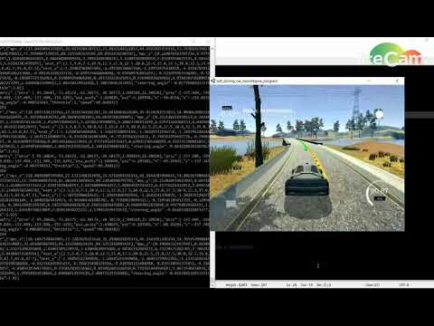
Please Click on the images to progress to the YouTube video.