Using the IMOS User Code Library with Python
Table of Contents
- 1. Introduction
- 2. General Features of the netCDF4 module
-
3. Dataset examples
- 3.1 AATAMS – Animal Tagging and Monitoring - non QC'd data
- 3.2 DWM – Deep Water Moorings
- 3.3 ACORN – Ocean Radar - non QC'd data
- 3.4 ANFOG – Ocean Gliders - QC'd good data
- 3.5 ANMN – National Mooring Network - QC'd good data
- 3.6 AUV – Autonomous Underwater Vehicle - non QC'd data
- 3.7 Argo – Argo Floats Program - non QC'd data
- 3.8 FAIMMS – Wireless Sensor Networks - QC'd good data
- 3.9 SOOP – Ships Of Opportunity
- 3.10 SRS – Satellite Remote Sensing
This document intends to present how to load IMOS NetCDF data into a Python environment, and offers some suggestions about how to use the data once loaded. All the examples below will use the netCDF4 Python module (http://code.google.com/p/netcdf4-python/)
The examples provided in this document only represent a tiny bit of the content of most of the NetCDF files. There are usually many more variables available in a NetCDF file, and therefore many other ways to display data.
Each dataset-specific example below can be found in the demos folder as a separate Python script.
The code library can be checked out using a Git client, or be downloaded as a zip file : https://github.com/aodn/imos-user-code-library/archive/master.zip
The examples rely on the following Python packages, which need to be installed:
- numpy – standard package for scientific computing in Python, provides versatile numerical array objects (http://www.numpy.org/).
- matplotlib – for plotting (http://matplotlib.org/).
- netCDF4 – for accessing netCDF files (http://code.google.com/p/netcdf4-python/, follow the Documentation link for installation instructions).
The examples below have been tested in Python 2.7.3, with numpy 1.6.1, matplotlib 1.1.1, and version 1.0.2 of netCDF4. Later versions of these packages will usually work. Earlier versions may work also.
In order to find a dataset you are interested in, please refer to the portal help: http://help.aodn.org.au/help/?q=node/6. This is a how-to guide that can help users find an IMOS NetCDF file. When downloading your chosen dataset from the portal, choose one of the download options “List of URLs”, or “All source NETCDF files” to obtain netCDF files.
For users who are already familiar with IMOS facilities and datasets, IMOS NetCDF files are also directly accessible via an OPeNDAP catalog at : http://thredds.aodn.org.au/thredds/catalog/IMOS/catalog.html
Most of the examples in the following sections use the ‘Data URL’ of a dataset. If you have downloaded your dataset from the portal, the data URL is the file path to the file on your local machine. If you are using the THREDDS catelog, the file does not have to be downloaded to your local machine first – the OPeNDAP data URL can be parsed into Python. The OPeNDAP data URL is found on the ‘OPeNDAP Dataset Access Form’ page (see http://help.aodn.org.au/help/?q=node/11), inside the box labelled ‘Data URL’ just above the ‘Global Attributes’ field.
Note: the list of URL’s generated by the IMOS portal when choosing that download option can be converted to a list of OPeNDAP data URL’s by replacing string http://data.aodn.org.au/IMOS/opendap with http://thredds.aodn.org.au/thredds/dodsC/IMOS.
The first step consists of opening a NetCDF file, whether this file is available locally or remotely on an OPeNDAP server.
Type in your Python command window (or script):
from netCDF4  import Dataset

aatams_URL = 'http://thredds.aodn.org.au/thredds/dodsC/IMOS/eMII/demos/AATAMS/marine_mammal_ctd-tag/2009_2011_ct64_Casey_Macquarie/ct64-M746-09/IMOS_AATAMS-SATTAG_TSP_20100205T043000Z_ct64-M746-09_END-20101029T071000Z_FV00.nc'
aatams_DATA = Dataset(aatams_URL)
This creates a netCDF Dataset object, through which you can access all the contents of the file.
Please refer to the netCDF4 module documentation for a complete description of the Dataset object::
'http://netcdf4-python.googlecode.com/svn/trunk/docs/netCDF4.Dataset-class.html'
(or type help(Dataset) at the Python prompt).
In order to see all the global attributes and some other information about the file, type in your command window:
print aatams_DATAThe output will look something like this:
 root group (NETCDF3_64BIT file format):
    project: Integrated Marine Observing System (IMOS)
    conventions: IMOS-1.2
    date_created: 2012-09-13T07:27:03Z
    title: Temperature, Salinity and Depth profiles in near real time
    institution: AATAMS
    site: CTD Satellite Relay Data Logger
    abstract: CTD Satellite Relay Data Loggers are used to explore how marine mammal behaviour relates to their oceanic environment. Loggers developped at the University of St Andrews Sea Mammal Research Unit transmit data in near real time via the Argo satellite system
    source: SMRU CTD Satellite relay Data Logger on marine mammals
…
    dimensions: obs, profiles
    variables: TIME, LATITUDE, LONGITUDE, TEMP, PRES, PSAL, parentIndex, TIME_quality_control, LATITUDE_quality_control, LONGITUDE_quality_control, TEMP_quality_control, PRES_quality_control, PSAL_quality_control
    groups:
Global attributes in the netCDF file become attributes of the Dataset object. A list of global attribute names is returned by the ncattrs() method of the object. The __dict__ attribute of the object is a dictionary of all netCDF attribute names and values.
# store the dataset's title in a local variable
title_str = aatams_DATA.title

# list all global attribute names
aatams_DATA.ncattrs()

# store the complete set of attributes in a dictionary (OrderedDict) object (similar to a standard Python dict, but
# maintains the order in which items are entered)
globalAttr = aatams_DATA.__dict__

# now you can also do (same effect as first command above)
title_str = globalAttr['title']To list all the variables available in the NetCDF file, type:
aatams_DATA.variables.keys()Output:
[u'TIME',
 u'LATITUDE',
 u'LONGITUDE',
 u'TEMP',
 u'PRES',
 u'PSAL',
 u'parentIndex',
 u'TIME_quality_control',
 u'LATITUDE_quality_control',
 u'LONGITUDE_quality_control',
 u'TEMP_quality_control',
 u'PRES_quality_control',
 u'PSAL_quality_control']
(The 'u' means each variable name is represented by a Unicode string.)
Each variable is accessed via a Variable object, in a similar way to the Dataset object. To access the Temperature variable :
# netCDF4 Variable object
TEMP = aatams_DATA.variables['TEMP']

# now you can print the variable's attributes and other info
print TEMP

# access variable attributes, e.g. its standard_name
TEMP.standard_name

# extract the data values (as a numpy array)
TEMP[:]

# the variable's dimensions (as a tuple)
TEMP.dimensionsThe Australian Animal Tagging And Monitoring System (AATAMS) is a coordinated marine animal tagging project. CTD Satellite Relay Data Loggers are used to explore how marine mammal behaviour relates to their oceanic environment.
NetCDF files can be found at : http://thredds.aodn.org.au/thredds/catalog/IMOS/AATAMS/marine_mammal_ctd-tag/catalog.html
In the example below, we demonstrate how to plot all the animal's dives as a single profile time-series of temperature, measured by a CTD tag.
To paste the code in your Python environment, please copy it from :
https://github.com/aodn/imos-user-code-library/blob/master/Python/demos/aatams.py
 Example of a Temperature Profile Time-series from AATAMS data

Example of a Temperature profile from AATAMS data
The Southern Ocean Time Series (SOTS) sub-facility provides high temporal resolution observations in sub-Antarctic waters. Observations are broad and include measurements of physical, chemical and biogeochemical parameters from multiple deep-water moorings.
NetCDF files can be found at : http://thredds.aodn.org.au/thredds/catalog/IMOS/DWM/SOTS/catalog.html
In the example below, the netCDF4 module is used to extract temperature data from a Pulse mooring instrument and print the abstract for the dataset. A temperature time series plot is produced using matplotlib.
To paste the code in your Python environment, please copy it from :
https://github.com/aodn/imos-user-code-library/blob/master/Python/demos/dwm.py
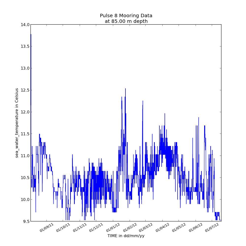
Temperature time-series from Pulse mooring
The Australian Coastal Ocean Radar Network (ACORN) facility comprises a coordinated network of HF radars delivering real-time, non-quality controlled and delayed-mode, quality controlled surface current data into a national archive.
NetCDF files can be found at : http://thredds.aodn.org.au/thredds/catalog/IMOS/ACORN/catalog.html
Monthly aggregated files are also available in the following folders: monthly_gridded_1h-avg-current-map_QC monthly_gridded_1h-avg-current-map_non-QC
In the example below, we plot the velocity field at a given time in a latitude / longitude grid.
To paste the code in your Python environment, please copy it from : https://github.com/aodn/imos-user-code-library/blob/master/Python/demos/acorn.py
 Example of Sea Water Speed gridded data with a velocity field from ACORN data
The Australian National Facility for Ocean Gliders (ANFOG), with IMOS/NCRIS funding, deploys a fleet of eight gliders around Australia.
NetCDF files can be found at : http://thredds.aodn.org.au/thredds/catalog/IMOS/ANFOG/seaglider/catalog.html
In the example below, we plot the salinity and depth time-series on the same graph. We select only the data points with a Quality Control flag of 1 (which means 'good data' , please refers to IMOS NetCDF User Manual for a description of the Quality Control flags, available at http://imos.org.au/facility_manuals.html)
To paste the code in your Python environment, please copy it from :
https://github.com/aodn/imos-user-code-library/blob/master/Python/demos/anfog.py
 Example of salinity and depth time-series from a SeaGlider deployment, filtered to plot good data only.
The Australian National Mooring Network Facility is a series of national reference stations and regional moorings designed to monitor particular oceanographic phenomena in Australian coastal ocean waters.
NetCDF files can be found at : http://thredds.aodn.org.au/thredds/catalog/IMOS/ANMN/catalog.html
In the example below, we plot the eastward current component measured with an ADCP instrument (in Western Australia).
To paste the code in your Python environment, please copy it from : https://github.com/aodn/imos-user-code-library/blob/master/Python/demos/anmn_adcp.py
 Example of a Sea Water Velocity plot from ADCP data
The IMOS Autonomous Underwater Vehicle (AUV) Facility operates an ocean going AUV called Sirius capable of undertaking high resolution, geo-referenced survey work.
NetCDF files can be found at : http://thredds.aodn.org.au/thredds/catalog/IMOS/AUV/catalog.html
In the example below, the netCDF4 module is used to extract depth, temperature, and time data and then produce a time-series plot showing the variation of water temperature and depth with time during the robot’s dive.
To paste the code in your Python environment, please copy it from : https://github.com/aodn/imos-user-code-library/blob/master/Python/demos/auv.py
 Example of a Temperature Time-series plot during an AUV dive
Argo floats have revolutionised our understanding of the broad scale structure of the oceans to 2000 m depth. In the past 10 years more high resolution hydrographic profiles have been provided by Argo floats then from the rest of the observing system put together. Each Argo float is identified by a unique identification number called a WMO ID.
NetCDF files can be found at : http://thredds.aodn.org.au/thredds/catalog/IMOS/Argo/aggregated_datasets/catalog.html
In the examples below, we plot Argo data from an aggregated file (one file per year per basin : Atlantic, Indian, Pacific North, Pacific South).
To paste the code in your Python environment, please copy it from : https://github.com/aodn/imos-user-code-library/blob/master/Python/demos/Argo.py

Example of a Sea Water Temperature profile from an Argo float
 Example of a Sea Water Temperature Time-series profile from an Argo float with its location over time
The IMOS Facility for Intelligent Monitoring of Marine Systems is a sensor network established in the Great Barrier Reef off the coast of Queensland, Australia. A 'sensor network' is an array of small, wirelessly interconnected sensors that collectively stream sensor data to a central data aggregation point. Sensor networks can be used to provide spatially dense bio-physical measurements in real-time.
NetCDF files can be found at : http://thredds.aodn.org.au/thredds/catalog/IMOS/FAIMMS/catalog.html
In the example below, we plot a temperature time-series using only data points with a quality control flag of 1 (which means 'good data', please refers to IMOS NetCDF User Manual for a description of the Quality Control, available at http://imos.org.au/facility_manuals.html).
To paste the code in your Python environment, please copy it from : https://github.com/aodn/imos-user-code-library/blob/master/Python/demos/faimms.py
 Example of a Sea Water Temperature at 5m depth on the Great Barrier Reaf from FAIMMS data
IMOS Ships of Opportunity Underway Expandable Bathythermographs (XBT) group is a research and data collection project working within the IMOS Ships of Opportunity Multi-Disciplinary Underway Network sub-facility.
NetCDF files can be found at : http://thredds.aodn.org.au/thredds/catalog/IMOS/SOOP/SOOP-XBT/catalog.html
In the example below, we first plot an individual XBT temperature profile, then plot all the profiles from a selected cruise.
To paste the code in your Python environment, please copy it from :
https://github.com/aodn/imos-user-code-library/blob/master/Python/demos/soop_xbt.py
 Example of Sea Water Temperature Profile from XBT data
 Example of Sea Water Temperature Time-series Profile from XBT data with the profiles location
The bio-optical data base underpins the assessment of ocean colour products in the Australian region (e.g. chlorophyll a concentrations, phytoplankton species composition and primary production).
NetCDF files can be found at : http://thredds.aodn.org.au/thredds/catalog/IMOS/SRS/BioOptical/catalog.html
In the example below, we plot a Chlorophyll-a profile (from High Performance Liquid Chromatography measurements of pigments in discrete sea-water samples).
To paste the code in your Python environment, please copy it from : https://github.com/aodn/imos-user-code-library/blob/master/Python/demos/srs_BioOptical_pigment.py
 Example of Pigment Data Profile from the BioOptical database dataset
The bio-optical data base underpins the assessment of ocean colour products in the Australian region (e.g. chlorophyll a concentrations, phytoplankton species composition and primary production).
NetCDF files can be found at : http://thredds.aodn.org.au/thredds/catalog/IMOS/SRS/BioOptical/catalog.html
In the example below, we plot the variation of Absorption coefficients of CDOM (gilvin) in discrete sea-water samples at different wavelengths and (2) the variation of absorption coefficients of CDOM at different wavelengths and different depths.
To paste the code in your Python environment, please copy it from : https://github.com/aodn/imos-user-code-library/blob/master/Python/demos/srs_BioOptical_absorption.py
 Example of Absorption Data plot from the BioOptical database dataset
 Example of Absorption Data at different depth from the BioOptical database dataset
Please refer to the SRS product Help page : http://help.aodn.org.au/help/?q=node/67
NetCDF files can be found at : http://thredds.aodn.org.au/thredds/dodsC/IMOS/SRS/GHRSST-SSTsubskin/
In the example below, we plot Sea Surface Temperature from a gridded data product.
Warning : this dataset can take a while to be loaded on your machine. If you plan to run this script multiple times, it would be faster to download the file first, and set the srs_L3P_URL to the file's location on your computer (see section 1.2 above).
To paste the code in your Python environment, please copy it from :
https://github.com/aodn/imos-user-code-library/blob/master/Python/demos/srs_l3p.py
 Example of Sea Surface Temperature plot from a L3P product centered on the GBR
Please refer to the SRS product Help page : http://help.aodn.org.au/help/?q=node/67
NetCDF files can be found at : http://thredds.aodn.org.au/thredds/dodsC/IMOS/SRS/SRS-SST/L3S-01day/
In the example below, we plot Sea Surface Temperature from a gridded data product
Warning : this dataset can take a while to be loaded on your machine. If you plan to run this script multiple times, it would be faster to download the file first, and set the srs_L3S_URL to the file's location on your computer (see section 1.2 above).
To paste the code in your Python environment, please copy it from :
https://github.com/aodn/imos-user-code-library/blob/master/Python/demos/srs_l3s.py
 Example of Sea Surface Temperature plot from a L3S product