mnist

Ground-up neural-network to classify MNIST handwritten digits, not bleeding edge by any definition

Dependencies

• Python 3.x
• Python libraries: numpy
• MNIST database from http://yann.lecun.com/exdb/mnist/ (plus uncompress) in local folder to code

Usage

There are two top-level programs that are intended for users to run: training.py and testing.py. The first can be used to build a neural network from scratch and train it on the MNIST training database; the second is used to test the performance of a given network against the MNIST test database, inspect the inner workings of the network and even test performance against your handwritten digits.

training.py

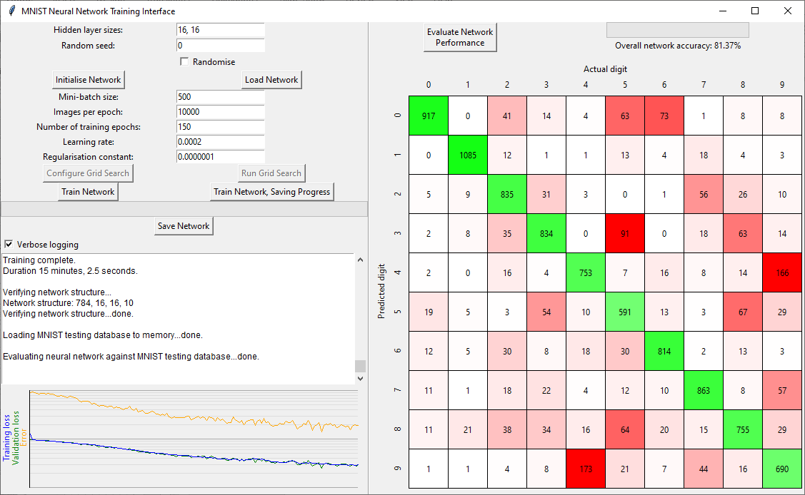
The training GUI is split into several areas as follows:

• Training parameters
• Logging
• Training graphs
• Network performance (confusion matrix)

To generate a trained network from scratch, first set the hidden layer size of the network that you would like and click Initialise Network. Alternatively, you can train a network loaded from a file by clicking Load Network (this could be a network that's already had some training applied).

The parameters available (should) represent the typical nomenclature for machine learning, default values give some performance of the network in a useful timeframe. Once happy with your initialised / loaded network and training parameters, click Train Network and the CPU intensive processing will start (defualt parameters take ~15 minutes on an 8th Gen. Core i5). You can train networks that have already been trained to some degree. Progress is indicated graphically and in the logging area (although, only for the latest training run).

The graphing area shows the loss for the training data and for (a random subset of) validation data (blue and green, respectively), plus a record of the network's current performance (measured as the classification error). All of these are on a log-scale for the y-axis. If everything is going well all three lines should decrease in value as they grow to the right during training, with the green and blue being approximately equal. If the change is negligible towards the end of training, that's indication that you've reached a (local) minimum in the training loss, and hence maximum of classification performance. Well done you.

At any time the program isn't actively processing, you can manually save your network (no clues for which button). This could be after training, or immediately upon initialisation.

After training is complete, the confusion matrix is calculated for the complete MNIST test database. Tooltips are provided if you hover over any of the numbers in the confusion matrix, which show the indices of the MNIST test images that fell into that classification box. You can also perform this calculation after initialisation or loading of a network to check performance.

testing.py

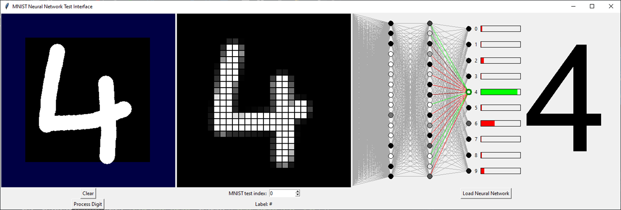
The testing GUI is simpler in operation compared to the training GUI. The left canvas area allows user graphical input, clicking Process Digit discretises the user's input into the middle area of the GUI. This shows the input in the standard 28x28 grid of the MNIST database. Alternatively, the user can use the numerical entry box to select one of the 10,000 MNIST test database images (perhaps to inspect some red boxes from the network's confusion matrix).

Load Neural Network brings a network into memory and graphically displays the structure. When a new user input or new MNIST example is selected, the forward calculation of the neural network is automatically produced. Neuron activations are shown with the colour of the circles, black is no activation, white is full activation. If the input is from the MNIST database, the output digit is colour coded (red/green) to indicate the success of the network for this example.

Clicking any neuron in the network highlights that neuron and all the connections leading directly into it. The bias of the neuron is now shown by the colour of the circle's border, green is very positive, red very negative, black is zero. The weights to the previous layer's neurons are also colour-coded by the same manner. If you select a neuron in the first hidden layer, the weights are drawn onto the discretised grid of input neurons. Studying these colours will no doubt lead to insight.

.nn file format

Describes a fully connected neural network, N layers (1<N<256). First layer has no weights and biases, input from external only.

Binary data, little endian

type	length	description
unsigned char	1	number of layers (N)
unsigned short	2	number of neurons in layer 0
unsigned short	2	number of neurons in layer 1
...	...	...
unsigned short	2	number of neurons in layer N-1
float	4	weight for neuron 0 in layer 1 to neuron 0 in layer 0
float	4	weight for neuron 0 in layer 1 to neuron 1 in layer 0
...	...	...
float	4	weight for neuron 0 in layer 1 to last neuron in layer 0
float	4	weight for neuron 1 in layer 1 to neuron 0 in layer 0
float	4	weight for neuron 1 in layer 1 to neuron 1 in layer 0
...	...	...
float	4	weight for neuron 1 in layer 1 to last neuron in layer 0
...	...	...
float	4	weight for last neuron in layer 1 to neuron 0 in layer 0
float	4	weight for last neuron in layer 1 to neuron 1 in layer 0
...	...	...
float	4	weight for last neuron in layer 1 to last neuron in layer 0
float	4	bias for neuron 0 in layer 1
float	4	bias for neuron 1 in layer 1
...	...	...
float	4	bias for last neuron in layer 1
float	4*x	above structure (weights, then biases) follows for each subsequent layer

Inspiration / References

• 3Blue1Brown's excellent series on Neural Networks (my original motivation to start this project)
• Stanford University's Andrew Ng's full course on Machine Learning
• Cambridge University's Mike Gordon's write up of going through a similar process
• Johannes Langelaar's exemplar Matlab code on the same topic, particularly helpful around the vector notation of the accumulators in the backpropagation algorithm